Safe Withdrawal Rates - Part 3: More Bootstrapping
In Part 2 of this series, As we saw in the previous post, the “standard” approach of choosing a safe withdrawal rate based on what has never failed in the past is questionable. The reason is that we simply don’t have that much data. If you had tried this approach in the past, by looking at what had never failed as of 1980, you would have overestimated the actual SWR and encountered a failure.
To try to address this, we used the stationary bootstrap to simulate alternate possible returns data. For each simulated data set, we re-ran the Trinity study methodology in order to see how different the “no failure” rate would have been. We found that in a non-trivial percentage of simulations, the “no failure” rate was much, much lower than the standard recommendations. This suggests that there is a fair degree of variability in what the Trinity study methodology could have reasonably found. So, just picking something that has never failed before does not give a good sense of how secure that withdrawal rate really is.
To do better, we’ll again turn to the stationary bootstrap. This time, we’ll use it to estimate safe withdrawal rates directly, rather than to study the statistical behavior of the Trinity study methodology.
For each possible duration and asset allocation, we generate 10,000 sequences of returns of the appropriate duration. Then, we compute the safe withdrawal rate for each return. From these 10,000 rates, we find the .001, .01, and .05 quantile. The results are summarized below:
| Safe withdrawal rates | ||||||||||
|---|---|---|---|---|---|---|---|---|---|---|
| 0.001 quantile | 0.01 quantile | 0.05 quantile | ||||||||
| 0% stocks | 15 years | 4.08% | 4.76% | 5.45% | ||||||
| 30 years | 1.89% | 2.27% | 2.78% | |||||||
| 45 years | 1.13% | 1.49% | 1.94% | |||||||
| 25% stocks | 15 years | 4.56% | 5.29% | 6.01% | ||||||
| 30 years | 2.34% | 2.84% | 3.42% | |||||||
| 45 years | 1.57% | 2.03% | 2.59% | |||||||
| 50% stocks | 15 years | 4.43% | 5.33% | 6.13% | ||||||
| 30 years | 2.39% | 2.98% | 3.70% | |||||||
| 45 years | 1.82% | 2.33% | 3.00% | |||||||
| 75% stocks | 15 years | 4.02% | 5.07% | 5.98% | ||||||
| 30 years | 2.13% | 2.91% | 3.73% | |||||||
| 45 years | 1.55% | 2.27% | 3.06% | |||||||
| 100% stocks | 15 years | 2.70% | 4.05% | 5.43% | ||||||
| 30 years | 1.39% | 2.28% | 3.32% | |||||||
| 45 years | 1.18% | 1.89% | 2.79% | |||||||
Remember, the .05 quantile is a value which 5% of the rates were less than (i.e. the 5th percentile). So, for the 0% stock allocation and 30 year duration, about 5% of the simulated runs had a SWR of less than 2.78%. One way to interpret this is that there’s about a 95% percent chance that a 2.78% withdrawal rate will succeed. As always with Monte Carlo methods like the bootstrap, this is dependent on the assumption that future results will match the distribution of historical returns.
The historical 2015 “no failure” rate discussed in Part 2 tends to lie between the .01 quantile and .05 quantiles here. Again, this underscores the fact that just applying the Trinity methodology naively will lead us to be overconfident about success rates!
What is an acceptable failure rate?
In order to use the above table, we need to decide on what an acceptable failure rate is. Going for a .1% failure rate comes at quite a cost in terms of how much we can withdraw. Looking at the 50% stocks and 30 year duration row, we have a 2.39% rate for .1% failure versus 2.98% for 1% failure. To achieve the same dollar amount of withdrawals, that means the .1% failure rate portfolio needs to be about 1.25x larger.
Keep in mind, a 45 year old American man has a .3% chance of dying in the next year1 alone. In light of that, hedging to keep withdrawal failures so low may seem slightly absurd.
We can get a better sense of the risk by plotting the cumulative probability of failure as we vary withdrawal rates. The figure below shows this for 50% stocks with 30 year duration:
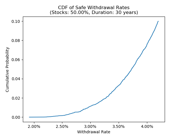
In this chart, the x-axis represents withdrawal rates, while the y-axis tells us the probability of failure with a given rate. As expected, this increases monotonically as the withdrawal rate goes up. The chart suggests that the failure rate remains fairly modest in the range of around 3%, but by the time we get up to a 4% withdrawal rate, it starts to increase rapidly.
Insights about asset allocation
As with our earlier bootstrapping results, the table above suggests that a high equity allocation may not be ideal. This is in contrast to the impression one might get from just studying classic Trinity style results. For the 45 year duration at the 1% failure rate level, 50% stocks gives a higher withdrawal rate than 75% or 100%. The gap between 50% and 75% are not large for most of these results, but the difference between 50% and 100% is quite substantial. That’s not surprising: given the higher volatility of stocks, it’s not implausible that we would see repeated sequences of bad returns in the simulated data. This leads me to believe that the 100% success rates of high equity allocations in the Trinity-style methodology are really the product of “luck”.
-
See the SSA life tables. ↩