Safe Withdrawal Rates - Part 4: Perpetual Withdrawal Rates
Recall from Part 1 that the Trinity study defined a withdrawal rate as “safe” so long as the portfolio always had enough to make withdrawals during retirement. That means if the portfolio was worth exactly $0 at the end of the retirement duration, that would count as a success. We’ve been using that same definition in the other parts of this series.
However, many retirees would not consider such an outcome a “success”. Watching your balance drop down closer and closer to 0 would be quite nerve-racking. Moreover, many people want to be able to leave assets to their heirs or charities upon their death.
There’s an easy (albeit conservative) way to adjust Trinity style safe withdrawal rates to guarantee a “minimum” floor for assets at death. Suppose the retiree has X dollars, and wishes to ensure that Y inflation-adjusted dollars will be available for heirs. They can simply put the Y dollars in an inflation-hedged instrument like TIPS or I-Bonds, which give a guaranteed real rate of return over inflation. Then, they can apply the usual SWR methodology to the remaining (X - Y) dollars.
However, setting an arbitrary “base” floor that assets should never dip below seems slightly arbitrary. What if we want to ensure that the whole principal remains in tact? In other words, what if we want a perpetual withdrawal rate that can last forever.
Let’s get one thing straight: if it is hard to estimate a withdrawal rate that is safe for 45 years, it is nearly impossible to figure out one that would last forever. All of the usual concerns about the small amount of data and the chance that future returns will be substantially different apply even more strongly. In fact, it’s safe to say that we do not have enough data, and future returns will be different. Nevertheless, it is interesting to see what the data we have suggests.
With that in mind, how should we estimate a perpetual rate? A common approach is to use something like the Trinity study methodology, but tweak the definition of success to require that the final portfolio value at the end of retirement at least as big as the starting value (or not too much smaller).
There are two problems with this approach, in my opinion. First of all, what duration length should we use? This approach leads to confusing results where a “longer” duration for the retirement leads us to a lower perpetual withdrawal rate. Consider a retirement duration of 1 year: even with a withdrawal rate of 0, there’s a significant chance that the portfolio will have dropped by a non-negligible amount after 1 year, just due to normal fluctuations of the market. The second problem is in deciding what the cut-off should be for how much of the initial portfolio should remain in order to count as a success. Most choices feel unprincipled and ad-hoc.
Solution: Monte Carlo simulation of long sequences of returns
The approach I prefer is to use Monte Carlo simulation (more precisely, the stationary bootstrap technique from Part 2) to generate very, very long sequences of returns. For each of these simulated returns, we’ll compute the safe withdrawal rate that would exactly deplete the principal after the end of the retirement duration. Of course, because this leaves the principal at 0 at the end, it is not in any sense a “perpetual rate”. But if the duration we consider is extremely long, then the rate is as plausibly perpetual as we can hope for, given the reality that the world will probably change dramatically over such a horizon. The benefit is that we thereby avoid ad-hoc choices seen in other attempts to answer this question.
By computing various quantiles of the withdrawal rates from our simulated results, we’ll be able to estimate what rates would lead to plausible success probabilities. (Again, subject to the usual caveats of Monte Carlo Simulation.)
The following table summarizes the results of 10,000 simulated returns for each asset allocation and duration:
| Safe Withdrawal Rates | ||||||||||
|---|---|---|---|---|---|---|---|---|---|---|
| 0.001 quantile | 0.01 quantile | 0.05 quantile | ||||||||
| 0% stocks | 100 years | 0.55% | 0.79% | 1.18% | ||||||
| 500 years | 0.38% | 0.63% | 1.01% | |||||||
| 1000 years | 0.34% | 0.62% | 0.99% | |||||||
| 25% stocks | 100 years | 0.97% | 1.43% | 1.96% | ||||||
| 500 years | 0.95% | 1.38% | 1.90% | |||||||
| 1000 years | 0.95% | 1.35% | 1.90% | |||||||
| 50% stocks | 100 years | 1.22% | 1.76% | 2.50% | ||||||
| 500 years | 1.20% | 1.75% | 2.46% | |||||||
| 1000 years | 1.21% | 1.78% | 2.41% | |||||||
| 75% stocks | 100 years | 1.27% | 1.85% | 2.65% | ||||||
| 500 years | 1.15% | 1.86% | 2.63% | |||||||
| 1000 years | 1.13% | 1.91% | 2.63% | |||||||
| 100% stocks | 100 years | 0.82% | 1.54% | 2.43% | ||||||
| 500 years | 0.80% | 1.47% | 2.35% | |||||||
| 1000 years | 0.88% | 1.52% | 2.43% | |||||||
For example, from this table, we see that a 50% stock allocation with a 1.21% withdrawal rate has an estimated 1 in 1000 failure rate for a 1000 year duration, because only 1 in 1000 trials had a safe withdrawal rate smaller than that.
Notice that the rates do not vary substantially as we go from 100, to 500, to 1000 year durations. The variation is at most a few tenths of a percent. Because of random fluctuations of Monte Carlo models, the 1000 year duration rate is even higher than the 500 year in some cases! This suggests that these rates are converging to something that really would last close to “indefinitely” under the assumptions of the model.
Below is the CDF plot for the 50% allocation over a 1000 year duration. The x-axis is the withdrawal rate, and the y-axis gives the probability of failure.
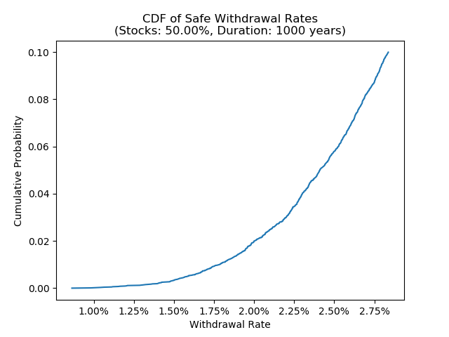
Altogether, with a moderate amount of stocks, we see that a withdrawal rate of between 1.75%-2% gives us a relatively small chance of failure over rather long durations. Given the length of these durations and the low failure rate, this seems like a reasonable estimate of a “perpetual withdrawal rate” – again, keeping in mind that we cannot hope to be certain that this will continue to work over a truly long period of time like a 1000 years.